Clifford data regression

CDR is an error mitigation method which predicts the noiseless value using training data, which can be generated by exact estimator such as a simulator and a noisy estimator such as a real device. The method consists of three steps:

(1) To generate noisless training data through efficient simulation using a classical computer, generate several approximate circuits in which non-Clifford gates are replaced by Clifford gates. Clifford gate can be configured with $H$, $S$, and CNOT gates. According to Gottesman-Knill theorem, quantum circuits consisting of Clifford gates can be efficiently simulated on a classical computer. A circuit containing non-Clifford gates can also be simulated using techniques derived from the Clifford circuit simulation method. However, the cost typically grows exponentially with the number of T gates. Therefore, reducing the number of T gates is essential to make the simulation feasible.

(2) The expectaion value $\langle O \rangle_\mathrm{noiseless}$ in a noiseless situation is calculated by using the generated approximate circuit, and the expectation value $\langle O \rangle_\mathrm{noisy}$ in a noisy situation is calculated by a noisy estimator such as a real device. This allows us to collect training data sets $\{(\langle O \rangle_\mathrm{noiseless}, \langle O \rangle_\mathrm{noisy}), \cdots\}$.

(3) For a given model $f(\langle O \rangle_\mathrm{noisy}, \boldsymbol{a})$, where $\boldsymbol{a} \in \mathbb{R}^m$ and $m$ is the number of parameters, optimize parameters $\boldsymbol{a}$ to minimize loss function $\sum_i\{f(\langle O \rangle_\mathrm{noisy}^i, \boldsymbol{a})-\langle O \rangle_\mathrm{noiseless}^i\}^2$. The trained model $f(\langle O \rangle_\mathrm{noisy}, \boldsymbol{a}_{\mathrm{opt}})$ returns noiseless expectation value for given noisy expectation value.

This technique is available even for large systems in the sense that Clifford+T circuits with moderate number of T gates can be simulated efficiently on a classical computer.

Prerequisite

QURI Parts modules used in this tutorial: quri-parts-algo, quri-parts-circuit, quri-parts-core and quri-parts-qulacs. You can install them as follows:

# !pip install "quri-parts[qulacs]"

Preparation and overview

Here, we prepare the circuit and the noise model we use throughout this tutorial. The circuit we use in this tutorial consists of an identity part and a non-trivial part. The non-trivial part is responsible for converting the state $|000\rangle$ into $\frac{1}{\sqrt{2}}\left(|000\rangle + |111\rangle\right)$, while we decompose the identity circuit into multiple gates to amplify the effect of the noises.

from quri_parts.circuit import QuantumCircuit
from quri_parts.circuit.utils.circuit_drawer import draw_circuit

qubit_count = 3

identity_circuit = QuantumCircuit(3)
identity_circuit.add_RX_gate(0, 1.3)
identity_circuit.add_RY_gate(1, 0.2)
identity_circuit.add_RZ_gate(0, -2.3)
identity_circuit.add_SqrtXdag_gate(1)
identity_circuit.add_T_gate(0)
identity_circuit.add_RX_gate(1, 0.4)
identity_circuit.add_RY_gate(0, 2.7)
identity_circuit.add_Tdag_gate(1)
identity_circuit.add_RY_gate(0, -2.7)
identity_circuit.add_T_gate(1)
identity_circuit.add_Tdag_gate(0)
identity_circuit.add_RX_gate(1, -0.4)
identity_circuit.add_RZ_gate(0, 2.3)
identity_circuit.add_SqrtX_gate(1)
identity_circuit.add_RX_gate(0, -1.3)
identity_circuit.add_RY_gate(1, -0.2)

circuit = QuantumCircuit(3)
circuit += identity_circuit
circuit.add_H_gate(0)
circuit.add_CNOT_gate(0, 1)
circuit.add_CNOT_gate(0, 2)


print("The circuit:")
draw_circuit(circuit, line_length=200)

#output
    The circuit:
       ___     ___     ___     ___     ___     ___     ___     ___     ___                  
      |RX |   |RZ |   | T |   |RY |   |RY |   |Tdg|   |RZ |   |RX |   | H |                 
    --|0  |---|2  |---|4  |---|6  |---|8  |---|10 |---|12 |---|14 |---|16 |-----●-------●---
      |___|   |___|   |___|   |___|   |___|   |___|   |___|   |___|   |___|     |       |   
       ___     ___     ___     ___     ___     ___     ___     ___             _|_      |   
      |RY |   |sXd|   |RX |   |Tdg|   | T |   |RX |   |sqX|   |RY |           |CX |     |   
    --|1  |---|3  |---|5  |---|7  |---|9  |---|11 |---|13 |---|15 |-----------|17 |-----|---
      |___|   |___|   |___|   |___|   |___|   |___|   |___|   |___|           |___|     |   
                                                                                       _|_  
                                                                                      |CX | 
    ----------------------------------------------------------------------------------|18 |-
                                                                                      |___| 

Then, we create a noise model with some NoiseInstructions. Here we consider BitFlipNoise and DepolarizingNoise.

from quri_parts.circuit.noise import (
    BitFlipNoise,
    DepolarizingNoise,
    NoiseModel,
)

noise_model = NoiseModel([
    BitFlipNoise(error_prob=0.01),
    DepolarizingNoise(error_prob=0.01),
])

Clifford data regression and peformance

Here, we explicitly show how to build an estimator that performs CDR. In this simple example, we will compare the performance of a CDR estimator with that of noiseless and noisy esimators. We first prepare an operator for this purpose.

from quri_parts.core.operator import Operator, pauli_label, PAULI_IDENTITY
op = Operator({
    pauli_label("Z0"): 0.25,
    pauli_label("Z1 Z2"): 2.0,
    pauli_label("X1 X2"): 0.5,
    pauli_label("Z1 Y2"): 1.0,
    pauli_label("X1 Y2"): 2.0,
    PAULI_IDENTITY: 3.0,
})

Next, we build a CDR estimator. In this example, the CDR estimator we create performs a quadratic regression using 10 data points, which corresponds to using 10 different training circuits. Each training circuit is constructed by ramdomly replacing 50% of the non-Clifford gates to clifford gates.

from quri_parts.algo.mitigation.cdr import create_cdr_estimator, create_polynomial_regression
from quri_parts.qulacs.estimator import (
    create_qulacs_density_matrix_concurrent_estimator,
    create_qulacs_vector_concurrent_estimator
)

noiseless_concurrent_estimator = create_qulacs_vector_concurrent_estimator()
noisy_concurrent_estimator = create_qulacs_density_matrix_concurrent_estimator(noise_model)
poly_regression = create_polynomial_regression(order=2)

cdr_estimator = create_cdr_estimator(
    noisy_estimator=noisy_concurrent_estimator,
    exact_estimator=noiseless_concurrent_estimator,
    regression_method=poly_regression,
    num_training_circuits=10,
    fraction_of_replacement=0.5
)

With the CDR estimator at hand, let's compare it's performance against the noiseless and noisy estimators.

from quri_parts.core.state import quantum_state
from quri_parts.qulacs.estimator import create_qulacs_vector_estimator, create_qulacs_density_matrix_estimator


state = quantum_state(qubit_count, circuit=circuit)

noiseless_estimator = create_qulacs_vector_estimator()
exact_estimate = noiseless_estimator(op, state)
print(f"Noiseless estimate: {exact_estimate.value}")

noisy_estimator = create_qulacs_density_matrix_estimator(noise_model)
noisy_estimate = noisy_estimator(op, state)
print(f"Noisy estimate: {noisy_estimate.value}")

cdr_estimate = cdr_estimator(op, state)
print(f"CDR estimate: {cdr_estimate.value}")

#output
    Noiseless estimate: (4.999999999999998+0j)
    Noisy estimate: (4.409201598385634+0j)
    CDR estimate: 5.001559956888837

Building the CDR estimator step by step

Now we start to explain all the steps necessary to construct a CDR estimator. This involves:

• Build a set of training circuits
• Collect data from the training ciricuits. The data is a sequence of noisy estimates and the corresponding noiseless estimates

$$\begin{equation} \{\left( \langle O \rangle _{\text{noisy}}, \langle O \rangle _{\text{noiseless}} \right), \cdots\} \end{equation}$$

• Pick a regression scheme to predict the noiseless result from noisy estimation of the noisy estimator.

Create training data

Next, we create training circuits and data. Training circuits are generated by replacing randomly chosen non-Clifford gates in the circuit with the closest Clifford gates. The number of non-Clifford gates determines the computational cost for Clifford+T simulator. Here, we generate 8 training circuits and each circuit has 6 non-Clifford gates.

After generating training circuit, we calculate the estimates for exact and noisy estimators.

from quri_parts.algo.mitigation.cdr import make_training_circuits

training_circuits = make_training_circuits(circuit, num_non_clifford_untouched=6, num_training_circuits=8)

for i, training_circuit in enumerate(training_circuits):
    print(f"training circuit: {i}")
    draw_circuit(training_circuit, line_length=200)

#output
    training circuit: 0
       ___     ___     ___     ___     ___     ___     ___     ___     ___                  
      |RX |   |RZ |   | S |   | Y |   | Y |   |Sdg|   | S |   |sXd|   | H |                 
    --|0  |---|2  |---|4  |---|6  |---|8  |---|10 |---|12 |---|14 |---|16 |-----●-------●---
      |___|   |___|   |___|   |___|   |___|   |___|   |___|   |___|   |___|     |       |   
       ___     ___     ___     ___     ___     ___     ___     ___             _|_      |   
      |RY |   |sXd|   |RX |   |Tdg|   | S |   |RX |   |sqX|   |UDF|           |CX |     |   
    --|1  |---|3  |---|5  |---|7  |---|9  |---|11 |---|13 |---|15 |-----------|17 |-----|---
      |___|   |___|   |___|   |___|   |___|   |___|   |___|   |___|           |___|     |   
                                                                                       _|_  
                                                                                      |CX | 
    ----------------------------------------------------------------------------------|18 |-
                                                                                      |___| 
    training circuit: 1
       ___     ___     ___     ___     ___     ___     ___     ___     ___                  
      |RX |   |Sdg|   | S |   | Y |   |RY |   |Tdg|   | S |   |sXd|   | H |                 
    --|0  |---|2  |---|4  |---|6  |---|8  |---|10 |---|12 |---|14 |---|16 |-----●-------●---
      |___|   |___|   |___|   |___|   |___|   |___|   |___|   |___|   |___|     |       |   
       ___     ___     ___     ___     ___     ___     ___     ___             _|_      |   
      |RY |   |sXd|   |UDF|   |Tdg|   | S |   |RX |   |sqX|   |UDF|           |CX |     |   
    --|1  |---|3  |---|5  |---|7  |---|9  |---|11 |---|13 |---|15 |-----------|17 |-----|---
      |___|   |___|   |___|   |___|   |___|   |___|   |___|   |___|           |___|     |   
                                                                                       _|_  
                                                                                      |CX | 
    ----------------------------------------------------------------------------------|18 |-
                                                                                      |___| 
    training circuit: 2
       ___     ___     ___     ___     ___     ___     ___     ___     ___                  
      |RX |   |Sdg|   | S |   |RY |   | Y |   |Sdg|   |RZ |   |sXd|   | H |                 
    --|0  |---|2  |---|4  |---|6  |---|8  |---|10 |---|12 |---|14 |---|16 |-----●-------●---
      |___|   |___|   |___|   |___|   |___|   |___|   |___|   |___|   |___|     |       |   
       ___     ___     ___     ___     ___     ___     ___     ___             _|_      |   
      |RY |   |sXd|   |UDF|   |Sdg|   | T |   |UDF|   |sqX|   |RY |           |CX |     |   
    --|1  |---|3  |---|5  |---|7  |---|9  |---|11 |---|13 |---|15 |-----------|17 |-----|---
      |___|   |___|   |___|   |___|   |___|   |___|   |___|   |___|           |___|     |   
                                                                                       _|_  
                                                                                      |CX | 
    ----------------------------------------------------------------------------------|18 |-
                                                                                      |___| 
    training circuit: 3
       ___     ___     ___     ___     ___     ___     ___     ___     ___                  
      |sqX|   |Sdg|   | T |   | Y |   |RY |   |Sdg|   | S |   |sXd|   | H |                 
    --|0  |---|2  |---|4  |---|6  |---|8  |---|10 |---|12 |---|14 |---|16 |-----●-------●---
      |___|   |___|   |___|   |___|   |___|   |___|   |___|   |___|   |___|     |       |   
       ___     ___     ___     ___     ___     ___     ___     ___             _|_      |   
      |RY |   |sXd|   |UDF|   |Tdg|   | T |   |UDF|   |sqX|   |RY |           |CX |     |   
    --|1  |---|3  |---|5  |---|7  |---|9  |---|11 |---|13 |---|15 |-----------|17 |-----|---
      |___|   |___|   |___|   |___|   |___|   |___|   |___|   |___|           |___|     |   
                                                                                       _|_  
                                                                                      |CX | 
    ----------------------------------------------------------------------------------|18 |-
                                                                                      |___| 
    training circuit: 4
       ___     ___     ___     ___     ___     ___     ___     ___     ___                  
      |sqX|   |RZ |   | S |   | Y |   |RY |   |Sdg|   |RZ |   |RX |   | H |                 
    --|0  |---|2  |---|4  |---|6  |---|8  |---|10 |---|12 |---|14 |---|16 |-----●-------●---
      |___|   |___|   |___|   |___|   |___|   |___|   |___|   |___|   |___|     |       |   
       ___     ___     ___     ___     ___     ___     ___     ___             _|_      |   
      |UDF|   |sXd|   |UDF|   |Tdg|   | T |   |UDF|   |sqX|   |UDF|           |CX |     |   
    --|1  |---|3  |---|5  |---|7  |---|9  |---|11 |---|13 |---|15 |-----------|17 |-----|---
      |___|   |___|   |___|   |___|   |___|   |___|   |___|   |___|           |___|     |   
                                                                                       _|_  
                                                                                      |CX | 
    ----------------------------------------------------------------------------------|18 |-
                                                                                      |___| 
    training circuit: 5
       ___     ___     ___     ___     ___     ___     ___     ___     ___                  
      |RX |   |RZ |   | S |   |RY |   | Y |   |Tdg|   | S |   |sXd|   | H |                 
    --|0  |---|2  |---|4  |---|6  |---|8  |---|10 |---|12 |---|14 |---|16 |-----●-------●---
      |___|   |___|   |___|   |___|   |___|   |___|   |___|   |___|   |___|     |       |   
       ___     ___     ___     ___     ___     ___     ___     ___             _|_      |   
      |RY |   |sXd|   |UDF|   |Tdg|   | S |   |UDF|   |sqX|   |UDF|           |CX |     |   
    --|1  |---|3  |---|5  |---|7  |---|9  |---|11 |---|13 |---|15 |-----------|17 |-----|---
      |___|   |___|   |___|   |___|   |___|   |___|   |___|   |___|           |___|     |   
                                                                                       _|_  
                                                                                      |CX | 
    ----------------------------------------------------------------------------------|18 |-
                                                                                      |___| 
    training circuit: 6
       ___     ___     ___     ___     ___     ___     ___     ___     ___                  
      |sqX|   |Sdg|   | T |   | Y |   |RY |   |Tdg|   | S |   |RX |   | H |                 
    --|0  |---|2  |---|4  |---|6  |---|8  |---|10 |---|12 |---|14 |---|16 |-----●-------●---
      |___|   |___|   |___|   |___|   |___|   |___|   |___|   |___|   |___|     |       |   
       ___     ___     ___     ___     ___     ___     ___     ___             _|_      |   
      |UDF|   |sXd|   |UDF|   |Sdg|   | T |   |RX |   |sqX|   |UDF|           |CX |     |   
    --|1  |---|3  |---|5  |---|7  |---|9  |---|11 |---|13 |---|15 |-----------|17 |-----|---
      |___|   |___|   |___|   |___|   |___|   |___|   |___|   |___|           |___|     |   
                                                                                       _|_  
                                                                                      |CX | 
    ----------------------------------------------------------------------------------|18 |-
                                                                                      |___| 
    training circuit: 7
       ___     ___     ___     ___     ___     ___     ___     ___     ___                  
      |RX |   |RZ |   | S |   | Y |   |RY |   |Sdg|   |RZ |   |sXd|   | H |                 
    --|0  |---|2  |---|4  |---|6  |---|8  |---|10 |---|12 |---|14 |---|16 |-----●-------●---
      |___|   |___|   |___|   |___|   |___|   |___|   |___|   |___|   |___|     |       |   
       ___     ___     ___     ___     ___     ___     ___     ___             _|_      |   
      |UDF|   |sXd|   |UDF|   |Sdg|   | T |   |RX |   |sqX|   |UDF|           |CX |     |   
    --|1  |---|3  |---|5  |---|7  |---|9  |---|11 |---|13 |---|15 |-----------|17 |-----|---
      |___|   |___|   |___|   |___|   |___|   |___|   |___|   |___|           |___|     |   
                                                                                       _|_  
                                                                                      |CX | 
    ----------------------------------------------------------------------------------|18 |-
                                                                                      |___| 

Noisy estimation on training circuits

exact_estimates = noiseless_concurrent_estimator(
    [op], [quantum_state(qubit_count, circuit=training_circuit) for training_circuit in training_circuits]
)
exact_estimates = [e.value.real for e in exact_estimates]

print("exact estimates:")
print(exact_estimates)

noisy_estimates = noisy_concurrent_estimator(
    [op], [quantum_state(qubit_count, circuit=training_circuit) for training_circuit in training_circuits]
)
noisy_estimates = [e.value.real for e in noisy_estimates]
print("noisy estimates:")
print(noisy_estimates)

#output
    exact estimates:
    [4.571368420223662, 4.725938607139674, 4.553399561554554, 4.840181114424471, 5.011915331184432, 4.671190940323665, 4.314567931739591, 4.335370993717824]
    noisy estimates:
    [4.1053636571491925, 4.233573548857111, 4.109449533963103, 4.2840278247817825, 4.402936220208613, 4.187134123532713, 3.921822410894969, 3.94079220528753]

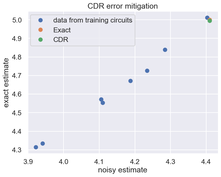
Define the regression function and get the mitigated value

Finally, we predict noiseless value by regression. QURI Parts has multiple options for regression. Here we perform second-order polynomial regression.

from quri_parts.algo.mitigation.cdr import (
    create_polynomial_regression,
)

poly_regression = create_polynomial_regression(order=2)

mitigated_val = poly_regression(
    noisy_estimate.value, noisy_estimates, exact_estimates
).real

print(f"mitigated value: {mitigated_val}")

#output
    mitigated value: 5.025232022296151

import matplotlib.pyplot as plt
import seaborn as sns

sns.set_theme("talk")
plt.rcParams["figure.figsize"] = (8, 6)
plt.plot(noisy_estimates, exact_estimates, "o", label="data from training circuits")
plt.plot(
    [noisy_estimator(op, state).value.real], [noiseless_estimator(op, state).value.real], "o",
    label="Exact"
)
plt.plot(
    [noisy_estimator(op, state).value.real], [cdr_estimator(op, state).value.real], "o",
    label="CDR"
)
plt.xlabel("noisy estimate")
plt.ylabel("exact estimate")
plt.title("CDR error mitigation")
plt.legend()
plt.show()

Create the CDR estimator

You can also create a CDR estimator that performs CDR behind the scenes. Once it's created, you can use it as a QuantumEstimator, which accepts Estimatable and QuantumState and returns Estimate.

from quri_parts.algo.mitigation.cdr import create_cdr_estimator

cdr_estimator = create_cdr_estimator(
    noisy_estimator=noisy_concurrent_estimator,
    exact_estimator=noiseless_concurrent_estimator,
    regression_method=poly_regression,
    num_training_circuits=10,
    fraction_of_replacement=0.5
)

estimate = cdr_estimator(op, state)
estimate

#output
    _Estimate(value=5.054745806576952, error=nan)