Quantum Fourier Transform

警告

In this tutorial, some circuits are constructed with the controlled_on option. This is the experimental multi-controlled circuit feature, which is not yet released in the latest version of QURI Parts.

Starting from this section, we demonstrate how to use QURI Parts to implement several algorithms containing quantum Fourier transform. We will cover:

• Period finding
• Phase estimation algorithm
• The Shor's algorithm

So, in this section, we first illustrate how to use QURI Parts to build the circuit for performing quantum Fourier transform.

The purpose of this section is two fold:

1. Introduce how multi-controlled gate feature is used in practice.
2. Fix the convention of quantum Fourier transform.

Quick review of the quantum Fourier transform

The quantum Fourier transform is defined by the following operation:

$$\begin{equation} |j \rangle \xrightarrow{\text{QFT}} \frac{1}{\sqrt{2^n}}\sum_{a=0}^{2^n - 1} \exp \left(i\frac{2\pi a j }{2^n}\right) |a \rangle, \end{equation}$$

where $n$ is the number of qubits. Written in terms of binary number notation, the above equation becomes:

$$\begin{equation} \begin{split} \text{QFT} |j_{n-1} \cdots j_0\rangle &= \frac{1}{\sqrt{2^n}} \sum_{\{a\}} \exp\left(2\pi i j \times [0.a_{n-1}\cdots a_0] \right) | a_{n-1} \cdots a_0 \rangle\\ &= \frac{1}{\sqrt{2^n}}\left( |0\rangle + e^{2\pi i 0.j_0}|1\rangle \right) \otimes \left( |0\rangle + e^{2\pi i 0.j_1 j_0}|1\rangle \right) \otimes \cdots \otimes \left( |0\rangle + e^{2\pi i 0.j_{n-1}\cdots j_0}|1\rangle \right), \end{split} \end{equation}$$

where $j = j_{n-1}\cdots j_0= \sum_{i=0}^{n-1} j_i 2^i$ and $\dfrac{a}{2^n} = 0.a_{n-1}\cdots a_0 = \sum_{i=0}^{n-1} a_i 2^{i-n}$.

The last line of eq.(2) gives a convenient form where the circuit representation of the operation can be read out straightforwardly. In our convention where the 0th qubit is positioned at the most right hand side, we need to first apply multiple SWAP gates to invert the order of the qubits:

$$\begin{equation} |j_{n-1} j_{n-2} \cdots j_1 j_0 \rangle \xrightarrow{\text{SWAPs}} |j_{0} j_{1} \cdots j_{n-2} j_{n-1} \rangle. \end{equation}$$

Then, we go through the standard textbook procedure of applying multiple controlled U1 gates to translate the above equation into the one in the second line of eq(2). For example, for the 0th qubit,

$$\begin{equation} \begin{split} &CU_{n-1, 0}(n) \cdots CU_{1, 0}(2) H_0|j_{0} j_{1} \cdots j_{n-2} j_{n-1} \rangle \\ =& \frac{1}{\sqrt{2}}CU_{n-1,0}(n) \cdots CU_{1, 0}(2) \sum_{k=0}^1 e^{2\pi i k\frac{ j_{n-1}}{2}}|j_{0} j_{1} \cdots j_{n-2} k \rangle \\ =& \frac{1}{\sqrt{2}}CU_{n-1,0}(n) \cdots CU_{2,0}(3) \sum_{k=0}^1 e^{2\pi i k (\frac{ j_{n-1}}{2} + \frac{ j_{n-2}}{2^2})}|j_{0} j_{1} \cdots j_{n-2} k \rangle \\ =& |j_{0} j_{1} \cdots j_{n-2}\rangle \otimes \frac{ |0\rangle + e^{2\pi i (0.j_{n-1} \cdots j_{0})}|1\rangle }{\sqrt{2}} \end{split} \end{equation}$$

where the notation $CU_{i,j}(k)$ denotes a controlled U1 gate with the i-th qubit as the controlled qubit and j-th qubit as the target index. The explicit matrix acting on the target qubit is

$$\begin{equation} U_j(k) = \begin{pmatrix} 1 & 0 \\ 0 & e^{\frac{2\pi i}{2^k}}\end{pmatrix}. \end{equation}$$

Repeating the procedure for the rest of the qubits will lead us to eq.(2).

Implement the quantum Fourier transform

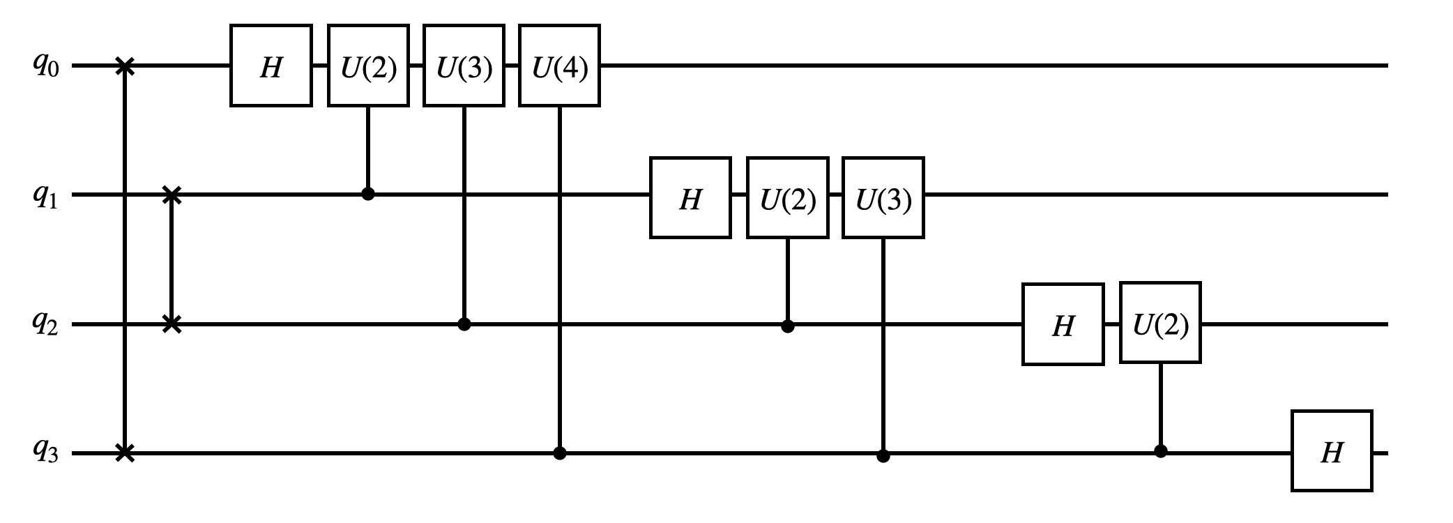
Now, we start to implement the circuit for quantum Fourier transform. As discussed in the last section, we first add sequence of SWAP gates to revert the qubit order. Then Hadamard gates and controlled U1 gates are added to perform the transformation. Here we show a diagram of a 4-qubit quantum Fourier transform circuit.

In QURI Parts, controlled U1 gates are created from U1 gates with the controlled_on argument specified.

from quri_parts.circuit import QuantumCircuit
circuit = QuantumCircuit(2)
circuit.add_U1_gate(0, lmd=0.5, controlled_on={1: 1})
circuit.gates[0]

#output
    QuantumGate(name='MultiControlledU1', target_indices=(0,), control_indices=(1,), controlled_on=(1,), classical_indices=(), params=(0.5,), pauli_ids=(), unitary_matrix=())

Now, we can put everything together and construct the circuit for quantum Fourier transform. The circuit for inverse Fourier tranform is also implemented by inverting the QFT circuit with quri_parts.circuit.inverse_circuit.

from quri_parts.circuit import QuantumCircuit, ImmutableQuantumCircuit, inverse_circuit
import numpy as np

def create_qft_circuit(qubit_count: int, inverse: bool = False) -> ImmutableQuantumCircuit:
    circuit = QuantumCircuit(qubit_count)
        
    for i in range(qubit_count//2):
        circuit.add_SWAP_gate(i, qubit_count-i-1)

    for target in range(qubit_count):
        circuit.add_H_gate(target)
        for l, control in enumerate(range(target+1, qubit_count)):
            angle = 2 * np.pi/2**(l+2)
            circuit.add_U1_gate(target, lmd=angle, controlled_on={control: 1})
    
    if inverse:
        return inverse_circuit(circuit).freeze()
    
    return circuit.freeze()

Let's check if the circuit we implemented is correct by looking at the circuit diagram of a 3-qubit quantum Fourier transform.

from quri_parts.circuit.utils.circuit_drawer import draw_circuit
print("Quantum Fourier transform on 3 qubits:")
draw_circuit(create_qft_circuit(3))

print("Inverse quantum Fourier transform on 3 qubits:")
draw_circuit(create_qft_circuit(3, inverse=True))

#output
    Quantum Fourier transform on 3 qubits:
                 ___     ___     ___                          
         0      | H |   |U1 |   |U1 |                         
    0 ----x-----|1  |---|2  |---|3  |-------------------------
          |     |___|   |___|   |___|                         
          |               |       |     ___      ___          
          |               |       |    | H |    |U1 |         
    1 ----|---------------●-------|----|4  |----|5  |---------
          |                       |    |___|    |___|         
          |                       |               |      ___  
          |                       |               |     | H | 
    2 ----x-----------------------●---------------●-----|6  |-
                                                        |___| 
    
    
    Inverse quantum Fourier transform on 3 qubits:
                                ___      ___     ___          
                               |U1 |    |U1 |   | H |    6    
    0 -------------------------|3  |----|4  |---|5  |-----x---
                               |___|    |___|   |___|     |   
                 ___     ___     |        |               |   
                |U1 |   | H |    |        |               |   
    1 ----------|1  |---|2  |----|--------●---------------|---
                |___|   |___|    |                        |   
         ___      |              |                        |   
        | H |     |              |                        |   
    2 --|0  |-----●--------------●------------------------x---
        |___|                                                 

Finally, let's confirm the circuit we implemented satisfies eq.(1).

from quri_parts.core.state import quantum_state, apply_circuit
from quri_parts.qulacs.simulator import evaluate_state_to_vector
import numpy as np
from numpy import pi, exp

n_qubits = 10
qft = create_qft_circuit(n_qubits)

for j in range(2**n_qubits):

    transformed = evaluate_state_to_vector(
        apply_circuit(qft, quantum_state(n_qubits, bits=j))
    ).vector

    expected = np.array(
        [exp(2j*pi*a*j / 2**n_qubits) for a in range(2**n_qubits)]
    ) / np.sqrt(2**n_qubits)

    assert np.allclose(transformed, expected)

The test passes successfully!

In the comming sections, we will embed the create_qft_circuit function above into various algorithms and show how QURI Parts can be used in the FTQC era.