Clifford data regression
CDRは、シミュレータのような厳密なestimatorと実機のようなノイズのあるestimatorによって生成される学習データを用��いて、ノイズのない値を予測するエラー軽減手法です。本手法は3つのステップから構成されます:
(1) 古典計算機を用いた効率的なシミュレーションによりノイズのない学習データを生成するため、非クリフォードゲートをクリフォードゲートに置き換えた近似回路を複数生成します。クリフォードゲートは、、およびCNOTゲートで構成することができます。Gottesman-Knillの定理によれば、クリフォードゲートで構成される量子回路は古典計算機で効率的にシミュレーションできます。非クリフォードゲートを含む回路も、クリフォード回路シミュレーション法から派生した技術を用いてシミュレーションすることができます。しかし、そのコストは通常、Tゲート数に応じて指数関数的に増大します。したがって、シミュレーションを実現可能にするためには、Tゲートの数を減らすことが不可欠です。
(2) ノイズなしのシチュエーションでの期待値は生成された近似回路を使用して計算され、ノイズありのシチュエーションでの期待値は実デバイスなどのノイズありのestimatorによって計算されます。これにより、訓練データセットを集めることができます。
(3) モデルを考え、損失関数を最小化するパラメータを求めます。ここではパラメータ、はパラメータの個数です。訓練されたモデルは与えられたノイズのある期待値に対してノイズのない期待値を返します。
この技術は、適度な数のTゲートを持つクリフォード+T回路を古典的なコンピュータで効率的にシミュレーションできるという意味で、大規模な系にも適用可能です。
前提条件
このチュートリアルで使用したQURI Partsモジュール:quri-parts-algo, quri-parts-circuit, quri-parts-core, quri-parts-qulacs
以下のようにインストールすることができます:
# !pip install "quri-parts[qulacs]"
準備と概要
ここでは、このチュートリアルで使用する回路とノイズモデルを準備します。このチュートリアルで使用する回路は、恒等パートと非自明パートで構成されています。非自明パートは状態をに変換する部分を担っている一方、ノイズの影響を増幅するために、恒等回路を複数のゲートに分解します。
from quri_parts.circuit import QuantumCircuit
from quri_parts.circuit.utils.circuit_drawer import draw_circuit

qubit_count = 3

identity_circuit = QuantumCircuit(3)
identity_circuit.add_RX_gate(0, 1.3)
identity_circuit.add_RY_gate(1, 0.2)
identity_circuit.add_RZ_gate(0, -2.3)
identity_circuit.add_SqrtXdag_gate(1)
identity_circuit.add_T_gate(0)
identity_circuit.add_RX_gate(1, 0.4)
identity_circuit.add_RY_gate(0, 2.7)
identity_circuit.add_Tdag_gate(1)
identity_circuit.add_RY_gate(0, -2.7)
identity_circuit.add_T_gate(1)
identity_circuit.add_Tdag_gate(0)
identity_circuit.add_RX_gate(1, -0.4)
identity_circuit.add_RZ_gate(0, 2.3)
identity_circuit.add_SqrtX_gate(1)
identity_circuit.add_RX_gate(0, -1.3)
identity_circuit.add_RY_gate(1, -0.2)

circuit = QuantumCircuit(3)
circuit += identity_circuit
circuit.add_H_gate(0)
circuit.add_CNOT_gate(0, 1)
circuit.add_CNOT_gate(0, 2)


print("The circuit:")
draw_circuit(circuit, line_length=200)
#output
    The circuit:
       ___     ___     ___     ___     ___     ___     ___     ___     ___
      |RX |   |RZ |   | T |   |RY |   |RY |   |Tdg|   |RZ |   |RX |   | H |
    --|0  |---|2  |---|4  |---|6  |---|8  |---|10 |---|12 |---|14 |---|16 |-----●-------●---
      |___|   |___|   |___|   |___|   |___|   |___|   |___|   |___|   |___|     |       |
       ___     ___     ___     ___     ___     ___     ___     ___             _|_      |
      |RY |   |sXd|   |RX |   |Tdg|   | T |   |RX |   |sqX|   |RY |           |CX |     |
    --|1  |---|3  |---|5  |---|7  |---|9  |---|11 |---|13 |---|15 |-----------|17 |-----|---
      |___|   |___|   |___|   |___|   |___|   |___|   |___|   |___|           |___|     |
                                                                                       _|_
                                                                                      |CX |
    ----------------------------------------------------------------------------------|18 |-
                                                                                      |___|
次に、いくつかのNoiseInstructionsを使ってノイズモデルを作成します。ここでは、BitFlipNoiseとDepolarizingNoiseを考えます。
from quri_parts.circuit.noise import (
    BitFlipNoise,
    DepolarizingNoise,
    NoiseModel,
)

noise_model = NoiseModel([
    BitFlipNoise(error_prob=0.01),
    DepolarizingNoise(error_prob=0.01),
])
Clifford data regressionの実行とそのパフォーマンス
ここでは、CDRを行うestimatorを構築する方法を明示的に示します。この簡単な例では、CDR estimatorの性能をノイズのないestimatorやノイズのあるestimatorと比較します。まず、この目的のために演算子を用意します。
from quri_parts.core.operator import Operator, pauli_label, PAULI_IDENTITY
op = Operator({
    pauli_label("Z0"): 0.25,
    pauli_label("Z1 Z2"): 2.0,
    pauli_label("X1 X2"): 0.5,
    pauli_label("Z1 Y2"): 1.0,
    pauli_label("X1 Y2"): 2.0,
    PAULI_IDENTITY: 3.0,
})
次に、CDR estimatorを作成します。この例では、作成したCDR estimatorは10個のデータポイントを用いて2次回帰を行いますが、これは10個の異なるトレーニング回路を用いることに相当します。各トレーニング回路は、非クリフォードゲートの50%をランダムにクリフォードゲートに置き換えることにより構築されます。
from quri_parts.algo.mitigation.cdr import create_cdr_estimator, create_polynomial_regression
from quri_parts.qulacs.estimator import (
    create_qulacs_density_matrix_concurrent_estimator,
    create_qulacs_vector_concurrent_estimator
)

noiseless_concurrent_estimator = create_qulacs_vector_concurrent_estimator()
noisy_concurrent_estimator = create_qulacs_density_matrix_concurrent_estimator(noise_model)
poly_regression = create_polynomial_regression(order=2)

cdr_estimator = create_cdr_estimator(
    noisy_estimator=noisy_concurrent_estimator,
    exact_estimator=noiseless_concurrent_estimator,
    regression_method=poly_regression,
    num_training_circuits=10,
    fraction_of_replacement=0.5
)
CDR estimatorを手にしたところで、ノイズのないestimatorとノイズのあ�るestimatorとの性能を比較してみよう。
from quri_parts.core.state import quantum_state
from quri_parts.qulacs.estimator import create_qulacs_vector_estimator, create_qulacs_density_matrix_estimator


state = quantum_state(qubit_count, circuit=circuit)

noiseless_estimator = create_qulacs_vector_estimator()
exact_estimate = noiseless_estimator(op, state)
print(f"Noiseless estimate: {exact_estimate.value}")

noisy_estimator = create_qulacs_density_matrix_estimator(noise_model)
noisy_estimate = noisy_estimator(op, state)
print(f"Noisy estimate: {noisy_estimate.value}")

cdr_estimate = cdr_estimator(op, state)
print(f"CDR estimate: {cdr_estimate.value}")
#output
    Noiseless estimate: (4.999999999999998+0j)
    Noisy estimate: (4.409201598385634+0j)
    CDR estimate: 5.001559956888837
CDR estimatorをステップバイステップで構築
ここで、CDR estimatorを構築するために必要なすべてのステップを説明します。ここでは以下を含みます:
- トレーニング回路の作成
- 各トレーニング回路からデータの収集。データはノイズありの推定値と、対応するノイズのない推定値
のシーケンスです。
- ノイズのある推定量からノイズのない結果を予測する回帰手法の選択
トレーニング回路の生成
まずは、トレーニング回路を生成します。トレーニング回路は、回路中のランダムに選ばれた非クリフォード・ゲートをそれに最も近いクリフォード・ゲートに置き換えることで生成されます。非クリフォードゲートの数によって、Clifford+Tシミュレータの計算コストが決まります。ここでは、8つのトレーニング回路を生成し、各回路には6つの非クリフォードゲートが残るように設定します。
トレーニング回路を生成した後、厳密な推定値とノイズありの推定値を計算します。
from quri_parts.algo.mitigation.cdr import make_training_circuits

training_circuits = make_training_circuits(circuit, num_non_clifford_untouched=6, num_training_circuits=8)

for i, training_circuit in enumerate(training_circuits):
    print(f"training circuit: {i}")
    draw_circuit(training_circuit, line_length=200)
#output
    training circuit: 0
       ___     ___     ___     ___     ___     ___     ___     ___     ___
      |RX |   |RZ |   | S |   | Y |   | Y |   |Sdg|   | S |   |sXd|   | H |
    --|0  |---|2  |---|4  |---|6  |---|8  |---|10 |---|12 |---|14 |---|16 |-----●-------●---
      |___|   |___|   |___|   |___|   |___|   |___|   |___|   |___|   |___|     |       |
       ___     ___     ___     ___     ___     ___     ___     ___             _|_      |
      |RY |   |sXd|   |RX |   |Tdg|   | S |   |RX |   |sqX|   |UDF|           |CX |     |
    --|1  |---|3  |---|5  |---|7  |---|9  |---|11 |---|13 |---|15 |-----------|17 |-----|---
      |___|   |___|   |___|   |___|   |___|   |___|   |___|   |___|           |___|     |
                                                                                       _|_
                                                                                      |CX |
    ----------------------------------------------------------------------------------|18 |-
                                                                                      |___|
    training circuit: 1
       ___     ___     ___     ___     ___     ___     ___     ___     ___
      |RX |   |Sdg|   | S |   | Y |   |RY |   |Tdg|   | S |   |sXd|   | H |
    --|0  |---|2  |---|4  |---|6  |---|8  |---|10 |---|12 |---|14 |---|16 |-----●-------●---
      |___|   |___|   |___|   |___|   |___|   |___|   |___|   |___|   |___|     |       |
       ___     ___     ___     ___     ___     ___     ___     ___             _|_      |
      |RY |   |sXd|   |UDF|   |Tdg|   | S |   |RX |   |sqX|   |UDF|           |CX |     |
    --|1  |---|3  |---|5  |---|7  |---|9  |---|11 |---|13 |---|15 |-----------|17 |-----|---
      |___|   |___|   |___|   |___|   |___|   |___|   |___|   |___|           |___|     |
                                                                                       _|_
                                                                                      |CX |
    ----------------------------------------------------------------------------------|18 |-
                                                                                      |___|
    training circuit: 2
       ___     ___     ___     ___     ___     ___     ___     ___     ___
      |RX |   |Sdg|   | S |   |RY |   | Y |   |Sdg|   |RZ |   |sXd|   | H |
    --|0  |---|2  |---|4  |---|6  |---|8  |---|10 |---|12 |---|14 |---|16 |-----●-------●---
      |___|   |___|   |___|   |___|   |___|   |___|   |___|   |___|   |___|     |       |
       ___     ___     ___     ___     ___     ___     ___     ___             _|_      |
      |RY |   |sXd|   |UDF|   |Sdg|   | T |   |UDF|   |sqX|   |RY |           |CX |     |
    --|1  |---|3  |---|5  |---|7  |---|9  |---|11 |---|13 |---|15 |-----------|17 |-----|---
      |___|   |___|   |___|   |___|   |___|   |___|   |___|   |___|           |___|     |
                                                                                       _|_
                                                                                      |CX |
    ----------------------------------------------------------------------------------|18 |-
                                                                                      |___|
    training circuit: 3
       ___     ___     ___     ___     ___     ___     ___     ___     ___
      |sqX|   |Sdg|   | T |   | Y |   |RY |   |Sdg|   | S |   |sXd|   | H |
    --|0  |---|2  |---|4  |---|6  |---|8  |---|10 |---|12 |---|14 |---|16 |-----●-------●---
      |___|   |___|   |___|   |___|   |___|   |___|   |___|   |___|   |___|     |       |
       ___     ___     ___     ___     ___     ___     ___     ___             _|_      |
      |RY |   |sXd|   |UDF|   |Tdg|   | T |   |UDF|   |sqX|   |RY |           |CX |     |
    --|1  |---|3  |---|5  |---|7  |---|9  |---|11 |---|13 |---|15 |-----------|17 |-----|---
      |___|   |___|   |___|   |___|   |___|   |___|   |___|   |___|           |___|     |
                                                                                       _|_
                                                                                      |CX |
    ----------------------------------------------------------------------------------|18 |-
                                                                                      |___|
    training circuit: 4
       ___     ___     ___     ___     ___     ___     ___     ___     ___
      |sqX|   |RZ |   | S |   | Y |   |RY |   |Sdg|   |RZ |   |RX |   | H |
    --|0  |---|2  |---|4  |---|6  |---|8  |---|10 |---|12 |---|14 |---|16 |-----●-------●---
      |___|   |___|   |___|   |___|   |___|   |___|   |___|   |___|   |___|     |       |
       ___     ___     ___     ___     ___     ___     ___     ___             _|_      |
      |UDF|   |sXd|   |UDF|   |Tdg|   | T |   |UDF|   |sqX|   |UDF|           |CX |     |
    --|1  |---|3  |---|5  |---|7  |---|9  |---|11 |---|13 |---|15 |-----------|17 |-----|---
      |___|   |___|   |___|   |___|   |___|   |___|   |___|   |___|           |___|     |
                                                                                       _|_
                                                                                      |CX |
    ----------------------------------------------------------------------------------|18 |-
                                                                                      |___|
    training circuit: 5
       ___     ___     ___     ___     ___     ___     ___     ___     ___
      |RX |   |RZ |   | S |   |RY |   | Y |   |Tdg|   | S |   |sXd|   | H |
    --|0  |---|2  |---|4  |---|6  |---|8  |---|10 |---|12 |---|14 |---|16 |-----●-------●---
      |___|   |___|   |___|   |___|   |___|   |___|   |___|   |___|   |___|     |       |
       ___     ___     ___     ___     ___     ___     ___     ___             _|_      |
      |RY |   |sXd|   |UDF|   |Tdg|   | S |   |UDF|   |sqX|   |UDF|           |CX |     |
    --|1  |---|3  |---|5  |---|7  |---|9  |---|11 |---|13 |---|15 |-----------|17 |-----|---
      |___|   |___|   |___|   |___|   |___|   |___|   |___|   |___|           |___|     |
                                                                                       _|_
                                                                                      |CX |
    ----------------------------------------------------------------------------------|18 |-
                                                                                      |___|
    training circuit: 6
       ___     ___     ___     ___     ___     ___     ___     ___     ___
      |sqX|   |Sdg|   | T |   | Y |   |RY |   |Tdg|   | S |   |RX |   | H |
    --|0  |---|2  |---|4  |---|6  |---|8  |---|10 |---|12 |---|14 |---|16 |-----●-------●---
      |___|   |___|   |___|   |___|   |___|   |___|   |___|   |___|   |___|     |       |
       ___     ___     ___     ___     ___     ___     ___     ___             _|_      |
      |UDF|   |sXd|   |UDF|   |Sdg|   | T |   |RX |   |sqX|   |UDF|           |CX |     |
    --|1  |---|3  |---|5  |---|7  |---|9  |---|11 |---|13 |---|15 |-----------|17 |-----|---
      |___|   |___|   |___|   |___|   |___|   |___|   |___|   |___|           |___|     |
                                                                                       _|_
                                                                                      |CX |
    ----------------------------------------------------------------------------------|18 |-
                                                                                      |___|
    training circuit: 7
       ___     ___     ___     ___     ___     ___     ___     ___     ___
      |RX |   |RZ |   | S |   | Y |   |RY |   |Sdg|   |RZ |   |sXd|   | H |
    --|0  |---|2  |---|4  |---|6  |---|8  |---|10 |---|12 |---|14 |---|16 |-----●-------●---
      |___|   |___|   |___|   |___|   |___|   |___|   |___|   |___|   |___|     |       |
       ___     ___     ___     ___     ___     ___     ___     ___             _|_      |
      |UDF|   |sXd|   |UDF|   |Sdg|   | T |   |RX |   |sqX|   |UDF|           |CX |     |
    --|1  |---|3  |---|5  |---|7  |---|9  |---|11 |---|13 |---|15 |-----------|17 |-----|---
      |___|   |___|   |___|   |___|   |___|   |___|   |___|   |___|           |___|     |
                                                                                       _|_
                                                                                      |CX |
    ----------------------------------------------------------------------------------|18 |-
                                                                                      |___|
トレーニング回路を使ったノイズあり・なしの期待値推定
exact_estimates = noiseless_concurrent_estimator(
    [op], [quantum_state(qubit_count, circuit=training_circuit) for training_circuit in training_circuits]
)
exact_estimates = [e.value.real for e in exact_estimates]

print("exact estimates:")
print(exact_estimates)

noisy_estimates = noisy_concurrent_estimator(
    [op], [quantum_state(qubit_count, circuit=training_circuit) for training_circuit in training_circuits]
)
noisy_estimates = [e.value.real for e in noisy_estimates]
print("noisy estimates:")
print(noisy_estimates)
#output
    exact estimates:
    [4.571368420223662, 4.725938607139674, 4.553399561554554, 4.840181114424471, 5.011915331184432, 4.671190940323665, 4.314567931739591, 4.335370993717824]
    noisy estimates:
    [4.1053636571491925, 4.233573548857111, 4.109449533963103, 4.2840278247817825, 4.402936220208613, 4.187134123532713, 3.921822410894969, 3.94079220528753]
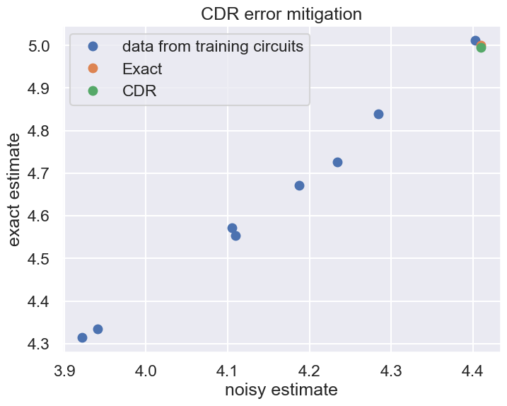
回帰関数を定義し、ノイズ緩和された値を取得
最後に、回帰によってノイズレス値を予測します。QURI Partsには回帰のための複数のオプションがあります。ここでは2次の多項式回帰を行います。
from quri_parts.algo.mitigation.cdr import (
    create_polynomial_regression,
)

poly_regression = create_polynomial_regression(order=2)

mitigated_val = poly_regression(
    noisy_estimate.value, noisy_estimates, exact_estimates
).real

print(f"mitigated value: {mitigated_val}")
#output
    mitigated value: 5.025232022296151
import matplotlib.pyplot as plt
import seaborn as sns

sns.set_theme("talk")
plt.rcParams["figure.figsize"] = (8, 6)
plt.plot(noisy_estimates, exact_estimates, "o", label="data from training circuits")
plt.plot(
    [noisy_estimator(op, state).value.real], [noiseless_estimator(op, state).value.real], "o",
    label="Exact"
)
plt.plot(
    [noisy_estimator(op, state).value.real], [cdr_estimator(op, state).value.real], "o",
    label="CDR"
)
plt.xlabel("noisy estimate")
plt.ylabel("exact estimate")
plt.title("CDR error mitigation")
plt.legend()
plt.show()
CDR estimatorの作成
通常のestimatorと同じように呼び出すだけで、裏でCDRを行うCDR estimatorを作成することもできます。
from quri_parts.algo.mitigation.cdr import create_cdr_estimator

cdr_estimator = create_cdr_estimator(
    noisy_estimator=noisy_concurrent_estimator,
    exact_estimator=noiseless_concurrent_estimator,
    regression_method=poly_regression,
    num_training_circuits=10,
    fraction_of_replacement=0.5
)

estimate = cdr_estimator(op, state)
estimate
#output
    _Estimate(value=5.054745806576952, error=nan)