Zero-noise extrapolation

ZNEは、複数のノイズレベル値に対応する期待値からノイズレスな値に対応する期待値を外挿する誤差軽減法です。この方法は3つのステップから構成されています:

(1) 元の回路の全体または一部を拡張してノイズレベルをスケーリングします。これにより、様々なノイズレベルを持つ複数の回路が得られます。最も単純なケースはノイズレベル3.0であり、以下のようになります。

$$U_{\text{original}} \rightarrow U_{\text{original}}U^{-1}_{\text{original}}U_{\text{original}}.$$

この回路は元のゲートの3倍のゲート数を持つので、これはノイズレベル3.0に相当すると考えられます。

(2) それぞれのノイズレベルに対応する期待値$\langle O(l)\rangle$を計算します。$l$はノイズレベルで$\langle O(l)\rangle$はノイズレベル $l$ における演算子$O$の期待値です。つまり、$l=1$はオリジナルの回路で、$l > 1.0$は拡張した回路に対応しています。

(3) 得たいのは期待値$\langle O(0)\rangle$であり、これはノイズがない時の期待値を指します。いくつかのノイズレベルで計算された複数の期待値を用いて、そこから外挿により推定します。

前提条件

このチュートリアルで使用するQURI Partsモジュール:quri-parts-algo, quri-parts-circuit, quri-parts-core, quri-parts-qulacs

以下のようにインストールすることができます:

!pip install "quri-parts[qulacs]"

準備と概要

ここでは、このチュートリアルで使用する回路とノイズモデルを準備します。このチュートリアルで使用する回路は、恒等パートと非自明パートで構成されています。非自明パートは状態$|000\rangle$を$\frac{1}{\sqrt{2}}\left(|000\rangle + |111\rangle\right)$に変換する部分を担っている一方、ノイズの影響を増幅するために、恒等回路を複数のゲートに分解します。

from quri_parts.circuit import QuantumCircuit
from quri_parts.circuit.utils.circuit_drawer import draw_circuit

qubit_count = 3

identity_circuit = QuantumCircuit(3)
identity_circuit.add_RX_gate(0, 1.3)
identity_circuit.add_RY_gate(1, 0.2)
identity_circuit.add_RZ_gate(0, -2.3)
identity_circuit.add_SqrtXdag_gate(1)
identity_circuit.add_T_gate(0)
identity_circuit.add_RX_gate(1, 0.4)
identity_circuit.add_RY_gate(0, 2.7)
identity_circuit.add_Tdag_gate(1)
identity_circuit.add_RY_gate(0, -2.7)
identity_circuit.add_T_gate(1)
identity_circuit.add_Tdag_gate(0)
identity_circuit.add_RX_gate(1, -0.4)
identity_circuit.add_RZ_gate(0, 2.3)
identity_circuit.add_SqrtX_gate(1)
identity_circuit.add_RX_gate(0, -1.3)
identity_circuit.add_RY_gate(1, -0.2)

circuit = QuantumCircuit(3)
circuit += identity_circuit
circuit.add_H_gate(0)
circuit.add_CNOT_gate(0, 1)
circuit.add_CNOT_gate(0, 2)


print("The circuit:")
draw_circuit(circuit, line_length=200)

#output
    The circuit:
       ___     ___     ___     ___     ___     ___     ___     ___     ___                  
      |RX |   |RZ |   | T |   |RY |   |RY |   |Tdg|   |RZ |   |RX |   | H |                 
    --|0  |---|2  |---|4  |---|6  |---|8  |---|10 |---|12 |---|14 |---|16 |-----●-------●---
      |___|   |___|   |___|   |___|   |___|   |___|   |___|   |___|   |___|     |       |   
       ___     ___     ___     ___     ___     ___     ___     ___             _|_      |   
      |RY |   |sXd|   |RX |   |Tdg|   | T |   |RX |   |sqX|   |RY |           |CX |     |   
    --|1  |---|3  |---|5  |---|7  |---|9  |---|11 |---|13 |---|15 |-----------|17 |-----|---
      |___|   |___|   |___|   |___|   |___|   |___|   |___|   |___|           |___|     |   
                                                                                       _|_  
                                                                                      |CX | 
    ----------------------------------------------------------------------------------|18 |-
                                                                                      |___| 

次に、いくつかのNoiseInstructionsを使ってノイズモデルを作成します。ここでは、BitFlipNoiseとDepolarizingNoiseを考えます。

from quri_parts.circuit.noise import (
    BitFlipNoise,
    DepolarizingNoise,
    NoiseModel,
)

noise_model = NoiseModel([
    BitFlipNoise(error_prob=0.01),
    DepolarizingNoise(error_prob=0.01),
])

ZNEの実行とそのパフォーマンスの確認

ここでは、ZNEを行うestimatorの構築方法を明示的に示します。この簡単な例では、ZNE estimatorの性能をノイズのないestimatorやノイズのあるestimatorと比較します。まず、この目的のために演算子を用意します。

from quri_parts.core.operator import Operator, pauli_label, PAULI_IDENTITY
op = Operator({
    pauli_label("Z0"): 0.25,
    pauli_label("Z1 Z2"): 2.0,
    pauli_label("X1 X2"): 0.5,
    pauli_label("Z1 Y2"): 1.0,
    pauli_label("X1 Y2"): 2.0,
    PAULI_IDENTITY: 3.0,
})

次に、ZNE estimatorを作成します。この例では、作成したZNE estimatorは3つのデータ点を用いて2次回帰を行いますが、これは3つの異なるスケールファクターを用いることに相当します。折り返されるゲートはランダムに選ばれます。ZNE estimatorを作成するには、まずノイズありのconcurrent estimatorが必要であることに注意してください。ここではQulacs density matrix concurrent estimatorを使用します。

from quri_parts.algo.mitigation.zne import create_polynomial_extrapolate, create_zne_estimator, create_folding_random
from quri_parts.qulacs.estimator import create_qulacs_density_matrix_concurrent_estimator

folding = create_folding_random()
scale_factors = [1.0, 2.0, 3.0]
poly_extrapolation = create_polynomial_extrapolate(order=2)
noisy_concurrent_estimator = create_qulacs_density_matrix_concurrent_estimator(noise_model)

zne_estimator = create_zne_estimator(
    noisy_concurrent_estimator, scale_factors, poly_extrapolation, folding
)

ZNE estimatorの結果を、ノイズあり・なしのestimatorの結果と比較してみましょう。

from quri_parts.qulacs.estimator import create_qulacs_density_matrix_estimator, create_qulacs_vector_estimator
from quri_parts.core.state import quantum_state

state = quantum_state(qubit_count, circuit=circuit)
noiseless_estimator = create_qulacs_vector_estimator()
noisy_estimator = create_qulacs_density_matrix_estimator(noise_model)

print("Noiseless estimate:", noiseless_estimator(op, state).value.real)
print("Noisy estimate:", noisy_estimator(op, state).value.real)
print("ZNE estimate:", zne_estimator(op, state).value)

#output
    Noiseless estimate: 4.999999999999998
    Noisy estimate: 4.409201598385634
    ZNE estimate: 4.633232349742287

ZNE estimatorをステップバイステップで構築

ここで、ZNE estimatorを構築するために必要なすべてのステップを説明します。ここでは以下のことを含みます：

• スケールファクターのリストから、スケーリングされた回路のリストを構築
• スケールした回路に対してノイズの多い推定を行うには、ノイズありconcurrent estimatorが必要です。そして、以下の一組のデータを得ます:

$$\begin{equation} \left\lbrace (\text{ScaleFactor}_0, \text{NoisyEstimation}_0), \cdots \right\rbrace \end{equation}$$

• ノイズありの期待値からノイズのない結果(ScaleFactor=0)を予測するための外挿方式を選択

スケーリングされた回路を作る

まずはスケーリングされた回路を作ります。回路を拡大縮小するには、scaling_circuit_foldingを使用します。QURI Partsには回路の折りたたみに複数のオプションがあります。ここではランダムフォールディングを使用します。

from quri_parts.algo.mitigation.zne import (
    create_folding_random,
    scaling_circuit_folding,
)

random_folding = create_folding_random()
scale_factors = [1.0, 2.0, 3.0]
scaled_circuits: list[QuantumCircuit] = []

for scale_factor in scale_factors:
    print("")
    print(f"{scale_factor = }")
    scaled_circuits.append(
        scaled_circuit:=scaling_circuit_folding(circuit, scale_factor, random_folding)
    )
    draw_circuit(scaled_circuit, line_length=800)

#output
    
    scale_factor = 1.0
       ___     ___     ___     ___     ___     ___     ___     ___     ___                  
      |RX |   |RZ |   | T |   |RY |   |RY |   |Tdg|   |RZ |   |RX |   | H |                 
    --|0  |---|2  |---|4  |---|6  |---|8  |---|10 |---|12 |---|14 |---|16 |-----●-------●---
      |___|   |___|   |___|   |___|   |___|   |___|   |___|   |___|   |___|     |       |   
       ___     ___     ___     ___     ___     ___     ___     ___             _|_      |   
      |RY |   |sXd|   |RX |   |Tdg|   | T |   |RX |   |sqX|   |RY |           |CX |     |   
    --|1  |---|3  |---|5  |---|7  |---|9  |---|11 |---|13 |---|15 |-----------|17 |-----|---
      |___|   |___|   |___|   |___|   |___|   |___|   |___|   |___|           |___|     |   
                                                                                       _|_  
                                                                                      |CX | 
    ----------------------------------------------------------------------------------|18 |-
                                                                                      |___| 
    
    scale_factor = 2.0
       ___     ___     ___     ___     ___     ___     ___     ___     ___     ___     ___     ___     ___     ___     ___     ___     ___     ___     ___                  
      |RX |   |RX |   |RX |   |RZ |   |RZ |   |RZ |   | T |   |Tdg|   | T |   |RY |   |RY |   |RY |   |RY |   |RY |   |RY |   |Tdg|   |RZ |   |RX |   | H |                 
    --|0  |---|1  |---|2  |---|6  |---|7  |---|8  |---|12 |---|13 |---|14 |---|18 |---|19 |---|20 |---|24 |---|25 |---|26 |---|28 |---|30 |---|32 |---|34 |-----●-------●---
      |___|   |___|   |___|   |___|   |___|   |___|   |___|   |___|   |___|   |___|   |___|   |___|   |___|   |___|   |___|   |___|   |___|   |___|   |___|     |       |   
       ___     ___     ___     ___     ___     ___     ___     ___     ___     ___     ___     ___     ___     ___     ___     ___                             _|_      |   
      |RY |   |RY |   |RY |   |sXd|   |sqX|   |sXd|   |RX |   |RX |   |RX |   |Tdg|   | T |   |Tdg|   | T |   |RX |   |sqX|   |RY |                           |CX |     |   
    --|3  |---|4  |---|5  |---|9  |---|10 |---|11 |---|15 |---|16 |---|17 |---|21 |---|22 |---|23 |---|27 |---|29 |---|31 |---|33 |---------------------------|35 |-----|---
      |___|   |___|   |___|   |___|   |___|   |___|   |___|   |___|   |___|   |___|   |___|   |___|   |___|   |___|   |___|   |___|                           |___|     |   
                                                                                                                                                                       _|_  
                                                                                                                                                                      |CX | 
    ------------------------------------------------------------------------------------------------------------------------------------------------------------------|36 |-
                                                                                                                                                                      |___| 
    
    scale_factor = 3.0
       ___     ___     ___     ___     ___     ___     ___     ___     ___     ___     ___     ___     ___     ___     ___     ___     ___     ___     ___     ___     ___     ___     ___     ___     ___     ___     ___                                                  
      |RX |   |RX |   |RX |   |RZ |   |RZ |   |RZ |   | T |   |Tdg|   | T |   |RY |   |RY |   |RY |   |RY |   |RY |   |RY |   |Tdg|   | T |   |Tdg|   |RZ |   |RZ |   |RZ |   |RX |   |RX |   |RX |   | H |   | H |   | H |                                                 
    --|0  |---|1  |---|2  |---|6  |---|7  |---|8  |---|12 |---|13 |---|14 |---|18 |---|19 |---|20 |---|24 |---|25 |---|26 |---|30 |---|31 |---|32 |---|36 |---|37 |---|38 |---|42 |---|43 |---|44 |---|48 |---|49 |---|50 |-----●-------●-------●-------●-------●-------●---
      |___|   |___|   |___|   |___|   |___|   |___|   |___|   |___|   |___|   |___|   |___|   |___|   |___|   |___|   |___|   |___|   |___|   |___|   |___|   |___|   |___|   |___|   |___|   |___|   |___|   |___|   |___|     |       |       |       |       |       |   
       ___     ___     ___     ___     ___     ___     ___     ___     ___     ___     ___     ___     ___     ___     ___     ___     ___     ___     ___     ___     ___     ___     ___     ___                             _|_     _|_     _|_      |       |       |   
      |RY |   |RY |   |RY |   |sXd|   |sqX|   |sXd|   |RX |   |RX |   |RX |   |Tdg|   | T |   |Tdg|   | T |   |Tdg|   | T |   |RX |   |RX |   |RX |   |sqX|   |sXd|   |sqX|   |RY |   |RY |   |RY |                           |CX |   |CX |   |CX |     |       |       |   
    --|3  |---|4  |---|5  |---|9  |---|10 |---|11 |---|15 |---|16 |---|17 |---|21 |---|22 |---|23 |---|27 |---|28 |---|29 |---|33 |---|34 |---|35 |---|39 |---|40 |---|41 |---|45 |---|46 |---|47 |---------------------------|51 |---|52 |---|53 |-----|-------|-------|---
      |___|   |___|   |___|   |___|   |___|   |___|   |___|   |___|   |___|   |___|   |___|   |___|   |___|   |___|   |___|   |___|   |___|   |___|   |___|   |___|   |___|   |___|   |___|   |___|                           |___|   |___|   |___|     |       |       |   
                                                                                                                                                                                                                                                       _|_     _|_     _|_  
                                                                                                                                                                                                                                                      |CX |   |CX |   |CX | 
    --------------------------------------------------------------------------------------------------------------------------------------------------------------------------------------------------------------------------------------------------|54 |---|55 |---|56 |-
                                                                                                                                                                                                                                                      |___|   |___|   |___| 

スケーリングされた回路の期待値のノイズあり推定

estimates = noisy_concurrent_estimator(
    [op], [quantum_state(qubit_count, circuit=scaled_circuit) for scaled_circuit in scaled_circuits]
)

for scale_factor, scaled_circuit, estimate in zip(scale_factors, scaled_circuits, estimates):
    print(
        f"scale factor {scale_factor}: {len(scaled_circuit.gates)=}, estimate: {estimate.value}"
    )

#output
    scale factor 1.0: len(scaled_circuit.gates)=19, estimate: (4.409201598385634+0j)
    scale factor 2.0: len(scaled_circuit.gates)=37, estimate: (4.099074907751645+0j)
    scale factor 3.0: len(scaled_circuit.gates)=57, estimate: (3.702852277840312+0j)

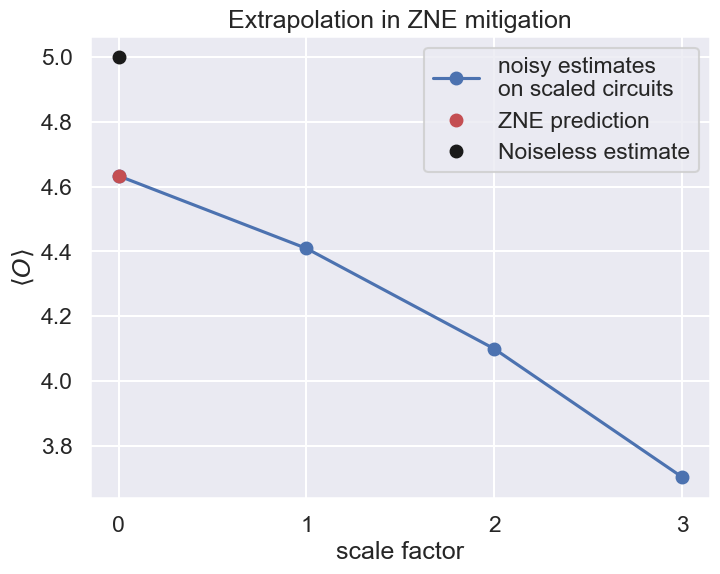
ゼロノイズ値の外挿

最後のステップは外挿です。QURI Partsには外挿のための複数のオプションがあります。ここでは2次の多項式外挿を使用します。

from quri_parts.algo.mitigation.zne import create_polynomial_extrapolate

poly_extrapolation = create_polynomial_extrapolate(order=2)
exp_vals = poly_extrapolation(scale_factors, [e.value for e in estimates])
print(f"mitigated estimate: {exp_vals}")

#output
    mitigated estimate: (4.633232349742287+0j)

import matplotlib.pyplot as plt
import seaborn as sns

sns.set_theme("talk")
plt.rcParams["figure.figsize"] = (8, 6)
plt.plot([0, *scale_factors], [exp_vals, *[e.value.real for e in estimates]], "-o", label="noisy estimates\non scaled circuits")
plt.plot([0], [exp_vals.real], "or", label="ZNE prediction")
plt.plot([0], [noiseless_estimator(op, state).value.real], "ok", label="Noiseless estimate")
plt.xlabel("scale factor")
plt.ylabel("$\\langle O \\rangle$")
plt.xticks([0, 1, 2, 3], [0, 1, 2, 3])
plt.title("Extrapolation in ZNE mitigation")
plt.legend()
plt.show()

ZNE estimatorの作成

通常のestimatorと同じように呼び出すだけで、裏で自動的にZNEを実行してノイズの影響を軽減した推定値を返すQuantumEstimatorを作成することもできます。

from quri_parts.algo.mitigation.zne import create_zne_estimator

zne_estimator = create_zne_estimator(
    noisy_concurrent_estimator, scale_factors, poly_extrapolation, random_folding
)

mitigated_estimate = zne_estimator(op, state)
mitigated_estimate.value

#output
    4.633232349742287